 Petko Aleksandrov
Educational content, not personalized advice. Nothing below accounts for your circumstances, tax position, or risk tolerance. Asset prices fall as well as rise, and cryptocurrency in particular can lose value rapidly and without warning.
The Short Answer
Dollar-cost averaging is an approach where you put a fixed sum into the same asset at set points on the calendar, regardless of whether prices are climbing or sliding. Your contribution stays constant while the number of units it buys varies: more units when quotes are low, fewer when they’re high. Over enough purchases, that produces a blended cost basis somewhere between the highest and lowest levels you paid.
What it doesn’t do is find good entry points. People conflate those two ideas constantly, and I’d rather clear that up in the first thirty seconds than three sections down.
An older version of this page mixed the concept with a chart-based buying method I was using at the time. Both approaches have their place, but they aren’t the same thing, so they now sit in separate sections.
Not a New Idea
Benjamin Graham described this technique in The Intelligent Investor back in 1949, decades before anyone applied it to cryptocurrency. Workplace retirement schemes have quietly operated on the same principle ever since: a percentage of salary buys units every payday, at whatever quote happens to prevail, with nobody consulted about conditions. Millions of people follow the approach without ever naming it. That history matters, I think, because it frames the method as ordinary long-term savings behavior rather than something clever, which is roughly the right way to hold it.
How the Mechanism Works
Four decisions define any plan of this kind:
- The asset; A single stock, an index fund, a basket of cryptocurrency, whatever you’ve settled on.
- The contribution: One fixed dollar amount, repeated.
- The frequency: Weekly, monthly, quarterly. Payday timing suits most people.
- The duration: Either a defined window, such as spreading a bonus across six months, or an open-ended commitment.
Then you follow it. That’s genuinely the whole method, and the discipline is harder than the arithmetic.
Notice what’s absent from that list: any judgment about valuation, momentum, news flow, or where the market might head next. Removing those judgments is the point. Regulators including FINRA publish investor education describing exactly this structure, largely because it reduces the number of decisions someone can get wrong.
A Worked Example
Three months, one hundred dollars each time, into an asset whose quote moves around:
| Month | Amount invested | Asset price | Units purchased |
| January | $100 | $10 | 10.00 |
| February | $100 | $8 | 12.50 |
| March | $100 | $12 | 8.33 |
| Total | $300 | 30.83 |
Divide total capital by total units: $300 divided by 30.83 gives roughly $9.73 per unit.
Here’s the part worth sitting with. Prices across those three months were $10, $8, and $12, which averages to $10 exactly. Yet the cost basis came out at $9.73, below that figure. Cheaper months bought disproportionately more units, which pulls the blended number down.
That effect isn’t magic, and it isn’t a guarantee of anything. It’s just what happens arithmetically when a constant sum meets a variable quote. Reverse the sequence, or run it through a market that only goes up, and the same mechanism works against you.
The Same Example in a Rising Market
Fair is fair. Run identical contributions through an asset that only appreciates, and the picture reverses completely:
| Month | Amount invested | Asset price | Units purchased |
| January | $100 | $10 | 10.00 |
| February | $100 | $12 | 8.33 |
| March | $100 | $15 | 6.67 |
| Total | $300 | 25.00 |
Cost basis lands at exactly $12.00 this time. Somebody who deployed the full three hundred dollars in January would instead hold thirty units rather than twenty-five, worth $450 against $375 by the end of March. Twenty percent behind, purely from waiting.
Neither table predicts anything. Both illustrate the same mechanical truth from opposite directions: gradual entry helps whenever quotes dip below your starting level and hurts whenever they don’t. Since most assets spend more time appreciating than falling across long horizons, the second scenario turns up more frequently than the first.
Why the Blended Cost Moves
Each new purchase gets weighted by how many units it bought, not by how much you spent. A hundred dollars deployed at $2 carries far more weight in the calculation than a hundred deployed at $20, because the first bought fifty units and the second bought five.
Which means:
- Volatile assets produce wider swings in unit counts, so the blending effect shows up more visibly.
- Steady assets barely benefit from the mechanism at all.
- A long decline followed by recovery is the scenario where this approach looks best in hindsight.
- Sustained appreciation from your starting point is the scenario where it looks worst.
What It’s Good For
- Removing timing decisions: Nobody knows where prices go next. Committing to a schedule means never having to form that opinion, which for most people is a net improvement over guessing.
- Behavioral protection: Panic-selling during a drop and buying enthusiastically during a rally is the documented pattern for retail participants. A schedule interrupts both impulses.
- Accessibility: Someone with a hundred dollars spare per month can build a position that would otherwise take years to save toward. Modern brokerages and exchanges support fractional purchases, which makes this practical in a way it wasn’t fifteen years ago.
- Reduced regret: Personally I find this the underrated benefit. Deploying everything the day before a twenty percent drop is psychologically brutal, and gradual entry softens that particular experience even when it costs performance.
Where It Falls Short
Honest limitations, since the internet has plenty of uncritical explanations already:
- Rising markets punish it: Money sitting in cash while an asset appreciates is money not appreciating. Studies published by large fund managers have generally found that immediate full deployment beat gradual entry across most historical periods, simply because assets rise more often than they fall. Worth reading one of those directly rather than taking my summary of it.
- No protection against permanent decline: Averaging into something that never recovers just means buying more of a losing position. The mechanism assumes eventual recovery, and that assumption fails for individual companies and plenty of cryptocurrency projects.
- Fee drag: Splitting one purchase into twelve means paying twelve fees, and flat-rate charges hurt small contributions badly.
- It’s not risk reduction: Spreading entry across time reduces exposure to one specific bad day. Your total exposure to the asset itself stays identical once fully invested.
- Record-keeping burden: Twelve purchases generate twelve cost-basis entries to track at disposal.
Which Assets Suit the Approach
| Asset type | Fit | Main consideration |
| Broad index fund | Strong | Recovery depends on whole markets rather than one business surviving |
| Sector or thematic funds | Moderate | Concentrated exposure, and a theme can stay unloved for years |
| Individual shares | Mixed | Nothing protects against a company that permanently fails |
| Cryptocurrency | Mixed | Extreme volatility magnifies the blending effect, though project failure is common |
| Bonds and cash equivalents | Weak | Limited variation leaves the mechanism little to work with |
Volatility is the ingredient that makes any of this worth discussing. An instrument that barely moves produces nearly identical unit counts at every purchase, so the blended figure ends up close to where a single deployment would have landed anyway. Which explains why the topic comes up constantly around crypto and almost never around money market holdings.
Compared With Investing Everything At Once
| Factor | Gradual contributions | Lump sum deployment |
| Timing exposure | Spread across several dates | Concentrated on one date |
| Historical performance | Weaker on average | Stronger on average |
| Worst-case entry | Softened | Fully exposed |
| Cash drag | Present until fully deployed | None |
| Emotional difficulty | Lower | Higher |
| Fee impact | Multiplied | Single charge |
Neither column wins outright. The mathematically stronger option and the psychologically sustainable option are frequently different options, and a plan you abandon in month four beats nothing at all by exactly zero.
Signal-Based Buying Is a Different Method
Some people, including me for a stretch around 2020, split capital into portions and then wait for chart conditions before deploying each one. Waiting for a counter-trend break, preferring assets already moving upward, trying to get each subsequent portion cheaper than the last: that describes a discretionary entry technique, not the systematic approach this page covers.
| Feature | Fixed-schedule contributions | Signal-based portions |
| Purchase timing | Predetermined dates | Technical conditions |
| Sum per purchase | Constant | Often variable |
| Response to price direction | Ignores it | Central to the decision |
| Primary objective | Remove timing judgment | Improve entry levels |
| Process type | Systematic | Discretionary |
| Exit approach | Separate consideration | Frequently uses profit targets |
Both can be defensible. Mixing their labels isn’t, because someone following a schedule expects consistency while someone reading charts expects to exercise judgment, and the two produce very different results in the same conditions.
Setting Up Recurring Purchases
Most platforms now automate this, which removes the willpower requirement entirely:
- Confirm your chosen venue supports scheduled buying for the specific asset. Coverage varies enormously between brokerages and crypto exchanges.
- Compare the fee structure for small repeat purchases against occasional larger ones. Check both the headline commission and any spread applied to the quote, since exchanges often bury cost in the second rather than the first.
- Set the amount at a level you can sustain through a bad quarter at work, not the level that feels ambitious today.
- Schedule contributions shortly after income arrives.
- Turn on statements or exports so cost-basis records accumulate automatically.
- Diarize a review, perhaps annually. Reviewing means checking whether the plan still fits your situation, not checking whether prices moved.
One small caution about automation: it works so well that people stop noticing what they own. Set a reminder to look properly at least once a year.
Fees, Records, and Tax
Fees deserve more attention than they usually get. A flat charge of a few dollars per purchase is trivial on a thousand-dollar contribution and punishing on a fifty-dollar one, so frequency and contribution size need to be chosen together rather than separately. Percentage-based charges scale more kindly, though spreads on cryptocurrency venues can quietly exceed the visible commission by a wide margin.
Record-keeping matters at the other end. Every purchase creates its own cost basis with its own date, and reconstructing twelve or thirty-six of those years later from memory is unpleasant. Export the history as you go.
On tax: treatment varies by jurisdiction and depends on whether a given transaction creates a disposal, a gain, or an income event. Some countries treat crypto-to-crypto exchanges as taxable disposals. Others apply holding-period rules that change the rate. Consult current guidance from your national tax authority or a qualified tax professional before assuming anything, and be aware that rules in this area have changed repeatedly since 2020.
An earlier version of this article included a specific claim about Bulgarian tax treatment. That claim has been removed pending verification, since jurisdiction-specific guidance shouldn’t sit unsourced on a page like this.
Frequently Asked Questions
Is dollar-cost averaging the same as averaging down?
No, and confusing them causes real damage. Averaging down means adding to a position that has already fallen, deliberately, because the lower quote looks attractive. Scheduled contributions happen on predetermined dates whether the asset rose, fell, or went nowhere. The distinction matters because averaging down concentrates capital into declining positions based on a judgment call, while a fixed schedule involves no judgment at all. One is discretionary; the other is mechanical.
How often should contributions happen?
Monthly suits most people, largely because income arrives monthly. Weekly contributions capture slightly more price variation but multiply fee events, which hurts when charges are flat rather than percentage-based. Quarterly reduces fee drag while leaving larger sums idle between purchases. Evidence for one frequency meaningfully beating another is thin, so the practical answer is whichever cadence you’ll actually maintain. Consistency contributes far more to the outcome than optimizing the interval ever will.
Can you use this approach to sell rather than buy?
Yes, and it’s sometimes called reverse or exit averaging. Instead of contributing fixed sums, you liquidate a fixed proportion or dollar value at set intervals, spreading disposal across several dates rather than picking one. Retirees drawing income and anyone unwinding a concentrated holding use this regularly. Same logic applies in reverse: you give up the chance of selling at the peak in exchange for avoiding the risk of selling everything at the bottom.
What’s the difference between this and value averaging?
Value averaging targets a portfolio value rather than a contribution size. You decide the balance should grow by, say, five hundred dollars monthly, then contribute whatever amount closes the gap, which means larger inputs after declines and smaller ones after gains. Occasionally it requires selling. That responsiveness can improve results mathematically, though it demands variable cash reserves and considerably more attention, so most people find the simpler fixed-contribution structure easier to sustain.
Does this work for individual stocks?
It can, but the assumption underneath gets shakier. Broad funds are diversified across many companies, so recovery from a downturn depends on the whole market rather than one business surviving. A single company can decline permanently, and contributing steadily into that decline compounds the damage. Anyone applying the method to individual names should size positions accordingly and accept that the mechanism offers no protection whatsoever against a company that simply fails.
Is it suitable for a small monthly budget?
Often yes, provided fees stay proportionate. Fractional purchasing lets modest sums buy partial units, which removes the old barrier of needing a full share price before participating. Watch for flat transaction charges, which can consume several percent of a small contribution before any price movement occurs. Platforms offering commission-free scheduled buying suit this situation better, though check whether the cost has simply moved into the quoted spread instead.
Does this guarantee I won’t lose money?
Definitely not, and any source suggesting otherwise is worth closing immediately. Spreading purchases across dates reduces the impact of one badly timed entry. It does nothing about the underlying asset declining, staying flat for a decade, or going to zero. Your eventual outcome depends primarily on what you bought and how long you held it, with entry timing contributing far less than most beginners assume. Losses remain entirely possible throughout.
Three Mistakes That Show Up Repeatedly
1. Pausing during declines: Halting contributions when quotes fall removes precisely the purchases that would lower your basis. Understandable, self-defeating.
2. Sizing from optimism: Committing more per interval than income comfortably supports leads to abandonment around month five, usually at the worst possible moment.
3. Treating the schedule as a substitute for research: Automation handles execution, never selection. Choosing badly and then buying that choice repeatedly just industrializes the error.
Summary
Fixed sums, fixed intervals, no opinions about direction required. That structure produces a blended cost basis, spreads timing exposure across multiple dates, and makes participation manageable for people who don’t have a large sum available today. It sacrifices some expected return in exchange for smoother experience and fewer decisions.
Whether that trade suits you depends on your horizon, your temperament, and how much cash is sitting idle in the meantime. Nobody can answer that from a webpage, including me.
Disclosure: This page provides general education only and does not constitute a recommendation to buy, sell, or hold any asset. Consider seeking guidance from a regulated professional before making decisions about your capital.